SWNE

Similarity Weighted Nonnegative Embedding (SWNE), is a method for visualizing high dimensional datasets. SWNE uses Nonnegative Matrix Factorization to decompose datasets into latent factors, projects those factors onto 2 dimensions, and embeds samples and key features in 2 dimensions relative to the factors. SWNE can capture both the local and global dataset structure, and allows relevant features to be embedded directly onto the visualization, helping with biological interpretation.

If you use SWNE in your research, please cite Wu et al, Cell Systems, 2018

Installation

Run the following code to install the package using devtools:

if(!require(remotes)){ install.packages("remotes") # If not already installed; }
remotes::install_github("linxihui/NNLM")
remotes::install_github("yanwu2014/swne")

If you want to run SWNE on chromatin accessibility data, install cisTopic as well.

devtools::install_github("aertslab/RcisTarget")
devtools::install_github("aertslab/AUCell")
devtools::install_github("aertslab/cisTopic")

Key Updates

*(10/21/2019): Improve SWNE embeddings by using PAGA graphs to prune the SNN graph. Update factor embedding distance function.

*(09/19/2019): The wrapper function RunSWNE now works on integrated Seurat datasets

*(05/15/2019): Updated all code and vignettes for Seurat V3 objects. Removed C1/snDropSeq projection vignette since it’s easier to use Seurat data integration (or CONOS)

Gene Expression Quickstart with Seurat

Download the example Seurat object which contains single cell RNA-seq profiles of 3000 PBMCs

## Load object
obj <- readRDS("Data/pbmc3k_final.RObj")

## Extract clusters
clusters <- obj$seurat_clusters

## Select genes to embed
genes.embed <- c("MS4A1", "GNLY", "CD3E", "CD14",
                 "FCER1A", "FCGR3A", "LYZ", "PPBP", "CD8A")

## Run SWNE
swne.embedding <- RunSWNE(obj, k = 16, genes.embed = genes.embed)

## Plot SWNE
PlotSWNE(swne.embedding, alpha.plot = 0.4, sample.groups = clusters,
         do.label = T, label.size = 3.5, pt.size = 1.5, show.legend = F,
         seed = 42)

Chromatin Accessibility Quickstart with cisTopic

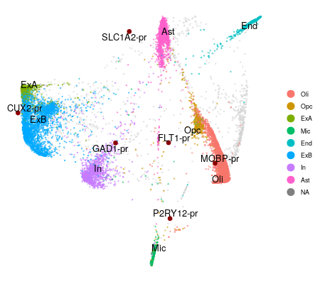
SWNE’s chromatin accessibility visualizations currently only work with cisTopic, a great method by Gonazalez-Blas et al that uses LDA to decompose scATAC or scTHS datasets. Download the example cisTopic object which contains single cell THS-seq profiles of 14,535 human brain cells from Lake, Sos, Chen et al, NBT, 2017.

library(cisTopic)
library(swne)
library(org.Hs.eg.db)
library(TxDb.Hsapiens.UCSC.hg38.knownGene)

## Load data
cisTopicObject <- readRDS("Data/adult-vCTX_cisTopic.RObj")

## Pull out clusters
clusters <- cisTopicObject@other$clusters

## Annotate regions
cisTopicObject <- getRegionsScores(cisTopicObject)
cisTopicObject <- annotateRegions(cisTopicObject, txdb = TxDb.Hsapiens.UCSC.hg38.knownGene,
                                  annoDb = "org.Hs.eg.db")

## Run SWNE embedding
swne.emb <- RunSWNE(cisTopicObject, alpha.exp = 1.25, snn.exp = 1, snn.k = 30)

## Embed genes based on promoter accessibility
marker.genes <- c("CUX2", "RORB", "FOXP2", "FLT1", "GAD1", "SST", "SLC1A2", "MOBP", "P2RY12")
swne.emb <- EmbedPromoters(swne.embedding, cisTopicObject, genes.embed = marker.genes,
                           peaks.use = NULL, alpha.exp = 1, n_pull = 3)

PlotSWNE(swne.emb, sample.groups = clusters, pt.size = 0.5, alpha.plot = 0.5, do.label = T,
         seed = 123)

scRNA-seq Walkthroughs and examples

Since SWNE is primarily meant for visualization and interpretation of the data, we typically use either Seurat or Pagoda2 as a primary scRNA-seq pipeline. All the R markdown files used to generate the walkthroughs can be found under the Examples/ directory.

1. A basic walkthrough using SWNE to visualize 3k PBMC cells starting from a pre-computed Seurat object
2. A basic walkthrough using SWNE to visualize 3k PBMC cells starting from a pre-computed Pagoda2 object
3. A basic walkthrough using SWNE to visualize 3k PBMC cells starting from a counts matrix
4. A walkthrough benchmarking SWNE against UMAP and SWNE using a large mouse hematopoiesis data from the Mouse Cell Atlas. The walkthrough was based of an analysis done by the UMAP authors in Figure 2 of their UMAP paper Becht, McInnes et al, NBT, 2019.
5. A walkthrough demonstrating SWNE on a hematopoiesis dataset and comparing SWNE against other embeddings including t-SNE and UMAP (recreating Figure 2 from our Cell Systems paper).
6. A walkthrough demonstrating SWNE on a single-cell study looking at Zika replication across time in a hepatoma cell line.
7. A walkthrough using SWNE to visualize four pancreas datasets that have undergone alignment with Seurat V3’s data integration.

scATAC/THS-seq Walkthroughs and examples

Since SWNE is primarily meant for visualization and interpretation of the data, we typically use either cisTopic as a primary pipeline

1. A walkthrough using SWNE to visualize a hematopoiesis trajectory that illustrates how to embed both the promoter accessibility of genes, and the binding site accessibility of transcription factors.

Recreating Figures

To recreate the figures from our preprint, see the Scripts/ directory.

To generate the simulated discrete and trajectory datasets, use splatter_generate.R. The simulated datasets we generated can be found here

To generate the visualizations and embedding evaluations, run splatter_discrete_swne.R and splatter_trajectory_swne.R for the discrete and trajectory simulations, respectively. To benchmark SWNE runtimes, use splatter_runtime_analysis.R.

The data needed to run hemato_swne.R can be found here and the raw data for the hematopoietic cells can be found, courtesy of the monocle2 developers, here. The hemato_swne.R script is also available as a SWNE walkthrough.

The data needed to run snDropSeq_swne.R on the cerebellar and visual cortex data can be found here and the raw data can be found at the GEO accession GSE97930.

The raw PBMC dataset can be found at the 10X genomics website.